 |
Open Qmin
0.8.0
GPU-accelerated Q-tensor-based liquid crystal simulations
|
 |
Open Qmin
0.8.0
GPU-accelerated Q-tensor-based liquid crystal simulations
|
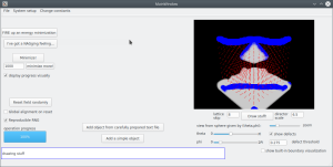
This repository contains code for performing lattice-discretized Landau deGennes liquid crystal modeling, using single or multiple CPU or GPU resources for efficient, large-scale simulations. Included is an optional graphical user interface for running and setting up the simulations. Usefully, the GUI has the functionality to generate a compilable file, allowing the GUI to be used for prototyping and then directly running larger- scale simulations.
Some doxygen documentation has been completed, but lots remains to be written. In any event, executing the command "doxygen doc/openQmin_documentation" from the root directory will produce a set of html documentation files.
See "INSTALLATION.md" for a few more details. Note that the "noQT" branch has stripped away all code related to the GUI for easy installation in environments without QT installed or where it is not necessary (e.g., on clusters)
build/openQminGUI.out
build/openQmin.out options...
For example, to run 100 FIRE minimization steps on a cubic lattice of side length 250:
build/openQmin.out -i 100 -l 250
To do the same thing but using a GPU in slot 0:
build/openQmin.out -i 100 -l 250 -g 0
To load a file, e.g. "asests/boundaryInput.txt" with custom boundaries prepared for a cubic lattice of side length 80
build/openQmin.out -i 100 -l 80 --boundaryFile assets/boundaryInput.txt
To do the above, but also save the post-minimization state:
./build/openQmin.out -i 80 --boundaryFile assets/boundaryInput.txt -l 80 --saveFile data/saveTesting
(for the above two lines, note that the file path is relative to where you currently are.)
As noted above, the "-l" command line flag can be used to specify the side length of a cubic simulation domain (other flags exist if you want the domain to be a rectangular prism). When using MPI to run a larger simulation domain, the default behavior is to take the command line size to specify the domain size ON EVERY MPI RANK. (One could imagine an alternate default behavior in which the command line specified the TOTAL size of the simulation domain, which was then divided among the different processors).
So, for example, the command:
mpirun -n 1 build/openQmin.out -l 100
will run execute a simulation domain of total size (100x100x100) lattice sites, on a single rank.
Moving to two processors, the command:
mpirun -n 2 build/openQmin.out -l 100
will run execute a simulation domain of total size (200x100x100) lattice sites, on two ranks (that is, each rank will control a 100x100x100 domain).
Similarly the command:
mpirun -n 8 build/openQmin.out -l 100
will run execute a simulation domain of total size (200x200x200) lattice sites, where each of the eight ranks continues to control a block of 100x100x100 lattice sites.
Both the command-line and gui exeecuutables can save the current configuration of the simulation, and simple visualization tools are available in the /visualizationTools directory to see the output of these systems. The output format is a simple txt file, where each line is: x y z Qxx Qxy Qxz Qyy Qyz t d, where x y z are the lattice site (in the case of MPI simulations, each rank will produce a separate file with x y z in absolute coordinates), followed by the current values of the Q tensor. The integer t specifies the "type" of the lattice site (bulk, boundary, part of an object), and d is a defect measure that is computed for all lattice sites not part of an object. By default this will be the largest eigenvalue of the Q tensor at that site; for lattice sites that are part of an object this will always be zero.
A separate header file exists in the main directory of the repository, "addObjectsToOpenQmin.h", which exists just to give the user a sense of how to add some of the pre-defined objects to the simulation. See the comments in that file for more details.
Both the command-line and gui versions of the executable have the ability to read in a user-prepared file that can specify objects composed of arbitrary collections of lattice sites and anchoring conditions (rather than just being limited to the predefined walls and colloids described in the addObjectsToOpenQmin.h file).
The input txt file specifying such objects must be very precisely formatted, and in the /tools/ directory we have included a simple utility to assist with this (although any other method can be used to generate the desired txt file, e.g. via python). A few examples of these custom boundary files are in the /assets/ directory; these were all created using the included mathematica notebook.
The formatting requirements are the following (copying from identical information provided in the comments of src/simulation/multirankSimulationBoundaries.cpp):
The first line must be a single integer specifying the number of objects to be read in. This is meant in the colloquial English sense, not in the zero-indexed counting sense. So, if you want your file to specify one object, make sure the first line is the number 1.
Each subsequent block must be formatted as follows (with no additional lines between the blocks): The first line MUST be formatted as a b c d where a=0 means oriented anchoring (such as homeotropic or oriented planar), a=1 means degenerate Planar b is a scalar setting the anchoring strength c is the preferred value of S0 d is an integer specifying the number of sites, N_B.
Subsequently, there MUST be N_b lines of the form x y z C1 C2 C3 C4 C5, where x, y, and z are the integer lattice sites, and C1, C2, C3, C4, C5 are real numbers corresponding to the desired anchoring conditions: For oriented anchoring, C1, C2, C3, C4, C5 correspond directly to the surface-preferred Q-tensor: C1 = Qxx, C2 = Qxy, C3=Qxz, C4 = Qyy, C5=Qyz, where one often will set the Q-tensor by choosing a locally preferred director, \nu^s, and setting Q^B = 3 S_0/2 * (\nu^s \nu^s - \delta{ab}/3).
For degenerate planar anchoring the five constants should be specified as, C1 = \hat{nu}x C2 = \hat{nu}y C3 = \hat{nu}z C4 = 0.0 C5 = 0.0, where \nu^s = {Cos[[Phi]] Sin[[theta]], Sin[[Phi]] Sin[[theta]], Cos[[theta]]} is the direction to which the LC should try to be orthogonal
Here are some convenient links to a variety of general information about the landau deGUI project; all of the below can also be accessed from the Project information tab (links work on the gitlab.io documenation website). Alternately, you can look at the markdown (.md) files in the base directory and the doc/markdown/ directories
 1.8.15